Accessing Fitted Model Objects
Source:vignettes/Accessing_Fitted_Model_Objects.Rmd
Accessing_Fitted_Model_Objects.RmdModels fitted with tidyfit (e.g. using the
regress() function) are stored in
tidyfit.models frames, which are tibbles that contain
information about multiple fitted models.
Individual fitted models are stored using the
tidyFit R6 class, in the
model_object column of the tidyfit.models
frame.
Here’s a simple example:
Suppose we want to fit a hierarchical features regression (HFR) — see here — for different shrinkage penalties. We begin by loading Boston house price data and fitting a regression for 4 different shrinkage parameters:
data <- MASS::Boston
mod_frame <- data |>
  regress(medv ~ ., m("hfr", kappa = c(0.25, 0.5, 0.75, 1))) |>
  unnest(settings)

# the tidyfit.models frame:
mod_frame
#> # A tibble: 4 × 7
#>   model estimator_fct `size (MB)` grid_id  model_object kappa weights
#>   <chr> <chr>               <dbl> <chr>    <list>       <dbl> <list>
#> 1 hfr   hfr::cv.hfr          1.23 #001|001 <tidyFit>     0.25 <NULL>
#> 2 hfr   hfr::cv.hfr          1.23 #001|002 <tidyFit>     0.5  <NULL>
#> 3 hfr   hfr::cv.hfr          1.23 #001|003 <tidyFit>     0.75 <NULL>
#> 4 hfr   hfr::cv.hfr          1.23 #001|004 <tidyFit>     1    <NULL>
The model_object columns contains 4 different models
(for different values of the parameter kappa). To extract
one of these models, we can use the get_tidyFit()
function:
# the tidyFit object:
get_tidyFit(mod_frame, kappa == 1)
#> <tidyFit> object
#>  method: hfr | mode: regression | fitted: yes
#>  no errors ✔ | no warnings ✔
Note that we can pass filters to ... (see
?get_tidyFit for more information).
The tidyFit class stores information necessary to obtain
predictions, coefficients or other information about the model and to
re-fit the model. It also contains the underlying model object (created
by hfr::cv.hfr in this case). To get this underlying
object, we can use the get_model() function:
# the underlying model:
hfr_model <- get_model(mod_frame, kappa == 0.75)
plot(hfr_model, kappa = 0.75)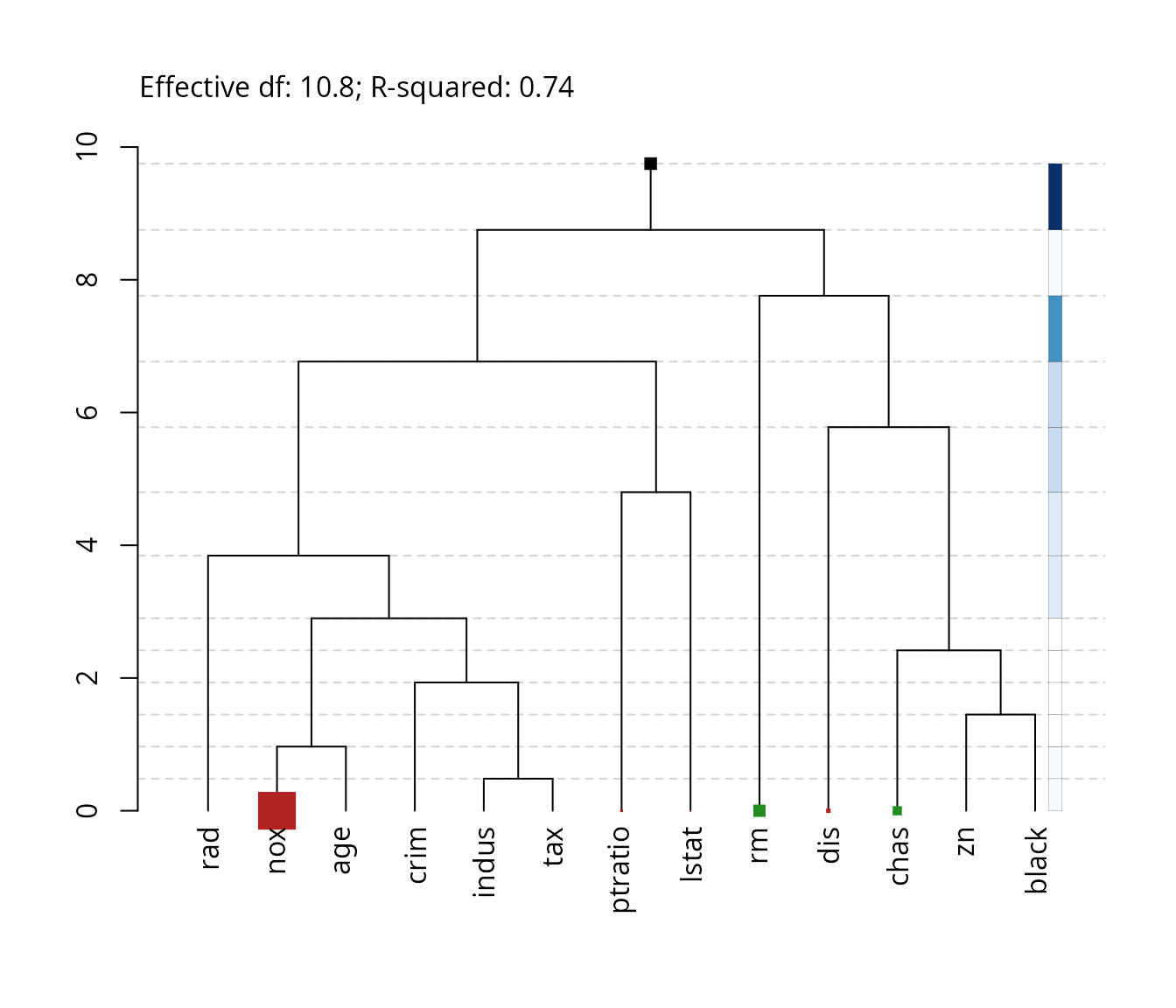
kappa defines the extent of shrinkage, with
kappa = 1 equal to an unregularized least squares (OLS)
regression, and kappa = 0.25 representing a regression
graph that is shrunken to 25% of its original size, with 25% of the
effective degrees of freedom. The regression graph is visualized using
the plot function.
Instead of extracting the underlying model, many generics can also be
applied directly to the tidyFit object as an added
convenience:
mod_frame |>
  get_tidyFit(kappa == .25) |>
  plot(kappa = .25)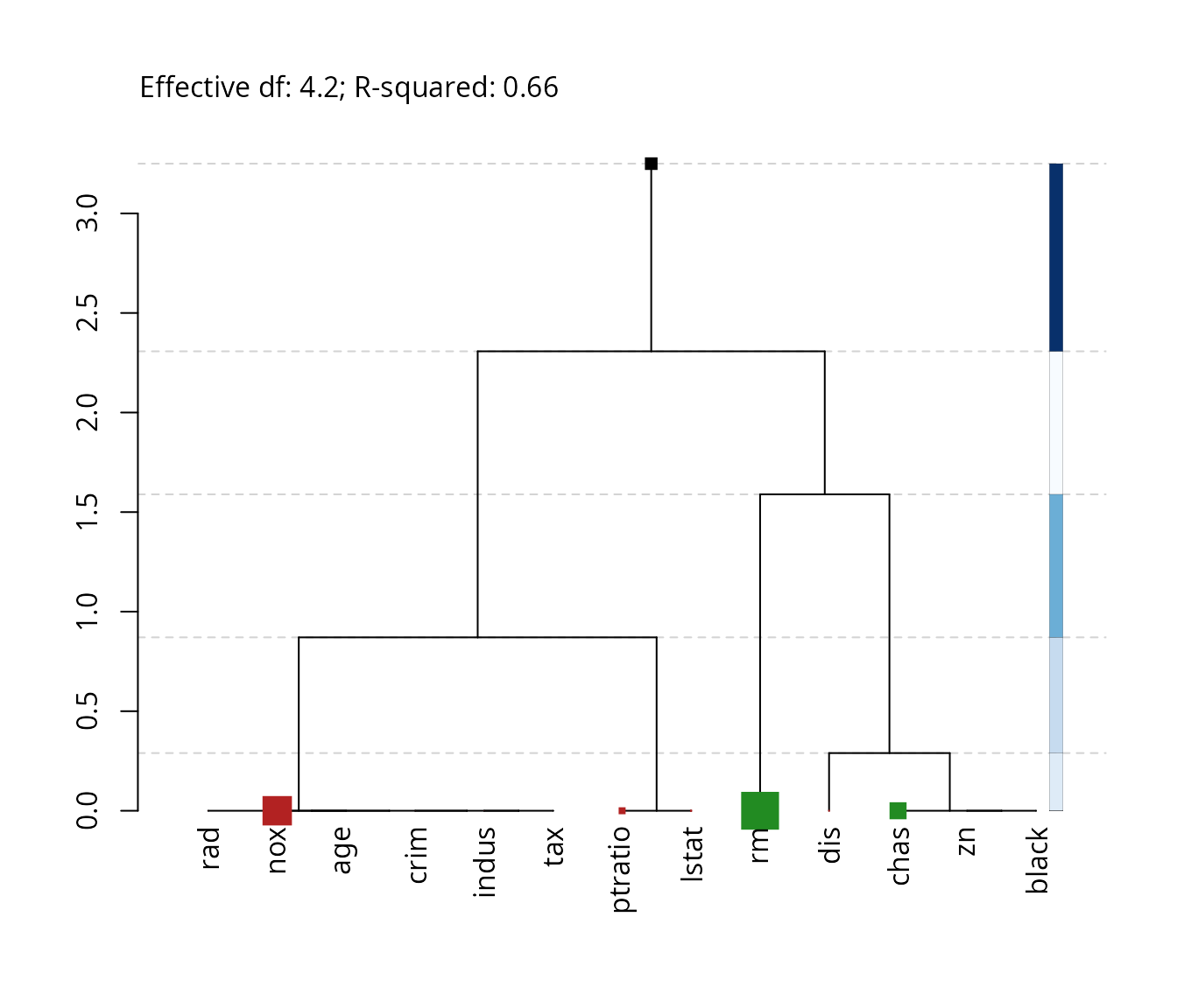
Finally, we can use pwalk to compare the different
settings in a plot:
# Store current par before editing
old_par <- par()

par(mfrow = c(2, 2))
par(family = "sans", cex = 0.7)
mod_frame |>
  arrange(desc(kappa)) |>
  select(model_object, kappa) |>
  pwalk(~plot(.x, kappa = .y,
              max_leaf_size = 2,
              show_details = FALSE))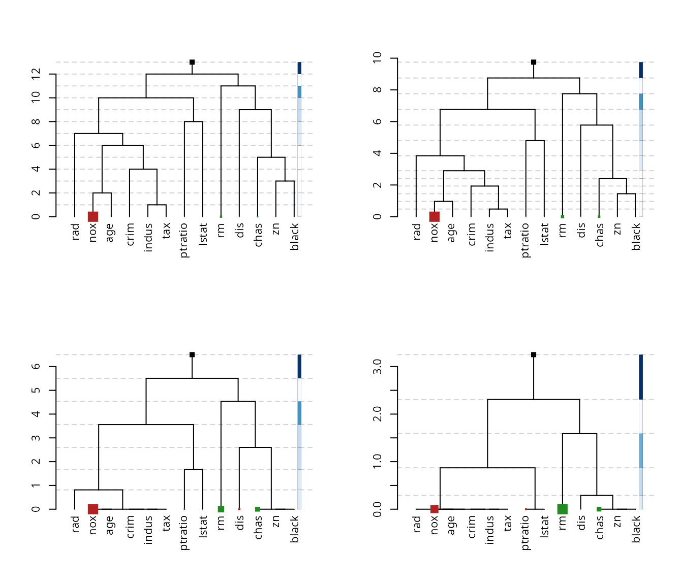
# Restore old par
par(old_par)
Notice how with each smaller value of kappa the height
of the tree shrinks and the model parameters become more similar in
size. This is precisely how HFR regularization works: it shrinks the
parameters towards group means over groups of similar features as
determined by the regression graph.