Bootstrapping Confidence Intervals • tidyfit

library(dplyr); library(tidyr); library(purrr); library(ggplot2) # Data wrangling
library(tidyfit) # Model fitting

The combination of .cv = "bootstraps" and .return_slices = TRUE in tidyfit::regress or tidyfit::classify makes it very easy to calculate bootstrap confidence intervals for estimated coefficients. As an additional convenience function, coef.tidyfit.models includes the option of adding percentile bootstrap intervals directly. In this short example, I will calculate and compare bootstrap confidence bands for a partial least squares regression and a principal components regression using Boston house price data:

data <- MASS::Boston |>
  scale() |>
  as_tibble()

tidyfit handles data scaling internally (i.e. PLSR and PCR are always fitted on scaled data), however, scaling the data manually here will give us standardized coefficients, which are easier to visualize and compare.

Fit the model

Instead of selecting an optimal number of latent components, I define a preset. This keeps things a little simpler. Note that dropping the ncomp = 5 argument results the optimal number of components being selected using bootstrap resampling.

model_frame <- data |>
  regress(medv ~ ., m("plsr", ncomp = 5), m("pcr", ncomp = 5),
          .cv = "bootstraps", .cv_args = list(times = 100), 
          .return_slices = TRUE)

The coefficients are returned for each slice when .add_bootstrap_intervals = FALSE (default behavior — see coef(model_frame)). To obtain bootstrap intervals, I pass .add_bootstrap_interval = TRUE to coef:

estimates <- coef(model_frame, 
                  .add_bootstrap_interval = TRUE, 
                  .bootstrap_alpha = 0.05)

estimates
#> # A tibble: 28 × 4
#> # Groups:   model [2]
#>    model term         estimate model_info      
#>    <chr> <chr>           <dbl> <list>          
#>  1 plsr  (Intercept) -0.000809 <tibble [1 × 3]>
#>  2 plsr  crim        -0.0698   <tibble [1 × 3]>
#>  3 plsr  zn           0.0940   <tibble [1 × 3]>
#>  4 plsr  indus       -0.0271   <tibble [1 × 3]>
#>  5 plsr  chas         0.0830   <tibble [1 × 3]>
#>  6 plsr  nox         -0.202    <tibble [1 × 3]>
#>  7 plsr  rm           0.295    <tibble [1 × 3]>
#>  8 plsr  age         -0.0148   <tibble [1 × 3]>
#>  9 plsr  dis         -0.333    <tibble [1 × 3]>
#> 10 plsr  rad          0.165    <tibble [1 × 3]>
#> # ℹ 18 more rows

The intervals are nested in model_info:

estimates <- estimates |>
  unnest(model_info)
estimates
#> # A tibble: 28 × 6
#> # Groups:   model [2]
#>    model term         estimate ncomp  .upper  .lower
#>    <chr> <chr>           <dbl> <dbl>   <dbl>   <dbl>
#>  1 plsr  (Intercept) -0.000809     5  0.0418 -0.0377
#>  2 plsr  crim        -0.0698       5  0.0564 -0.148 
#>  3 plsr  zn           0.0940       5  0.164   0.0240
#>  4 plsr  indus       -0.0271       5  0.0466 -0.0963
#>  5 plsr  chas         0.0830       5  0.142   0.0186
#>  6 plsr  nox         -0.202        5 -0.117  -0.302 
#>  7 plsr  rm           0.295        5  0.413   0.142 
#>  8 plsr  age         -0.0148       5  0.102  -0.107 
#>  9 plsr  dis         -0.333        5 -0.240  -0.432 
#> 10 plsr  rad          0.165        5  0.233   0.0758
#> # ℹ 18 more rows

Plot the results

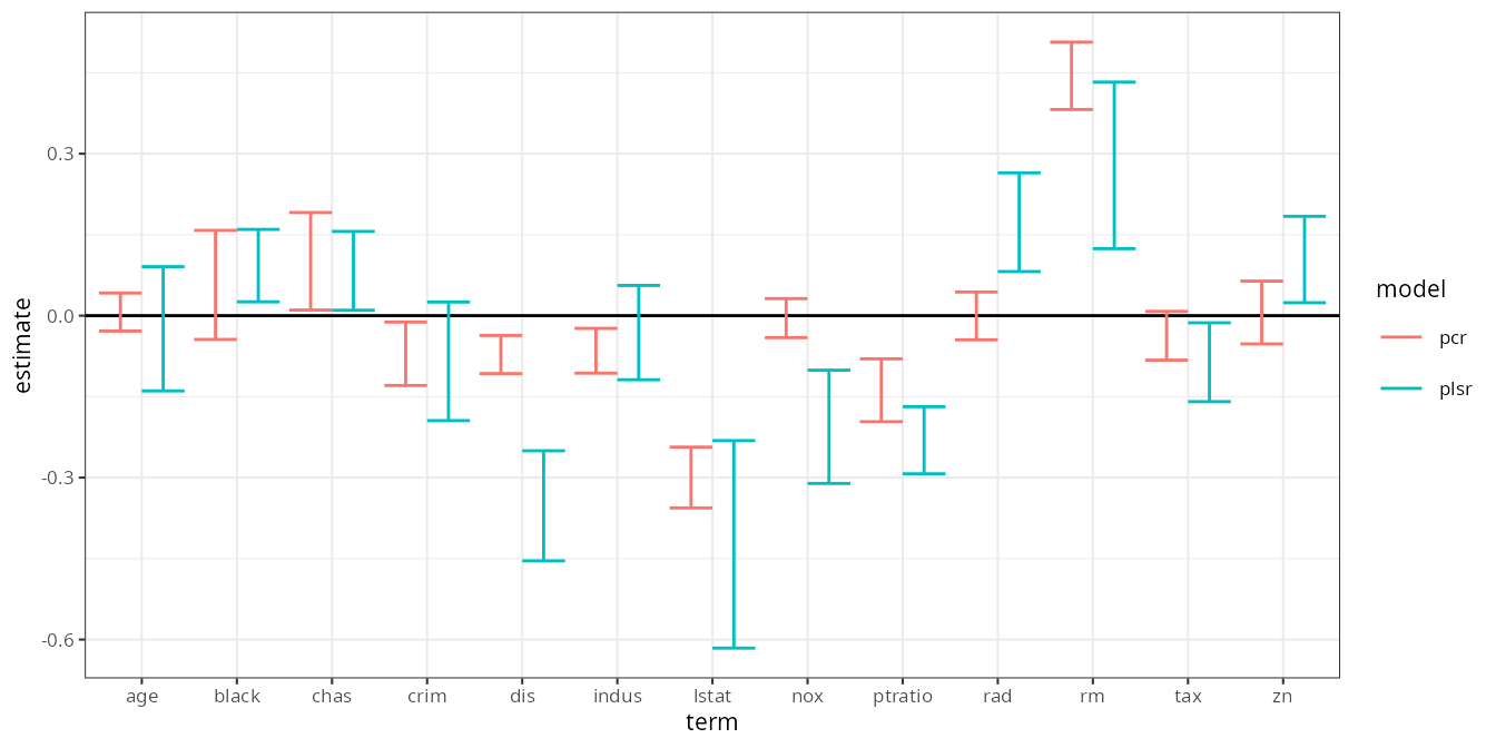
And thus, in a concise workflow, we have 95% bootstrap confidence intervals for the coefficients of a PCR and PLS regression:

estimates |>
  filter(term != "(Intercept)") |>
  ggplot(aes(term, estimate, color = model)) +
  geom_hline(yintercept = 0) +
  geom_errorbar(aes(ymin = .lower, ymax = .upper), position = position_dodge()) +
  theme_bw(8)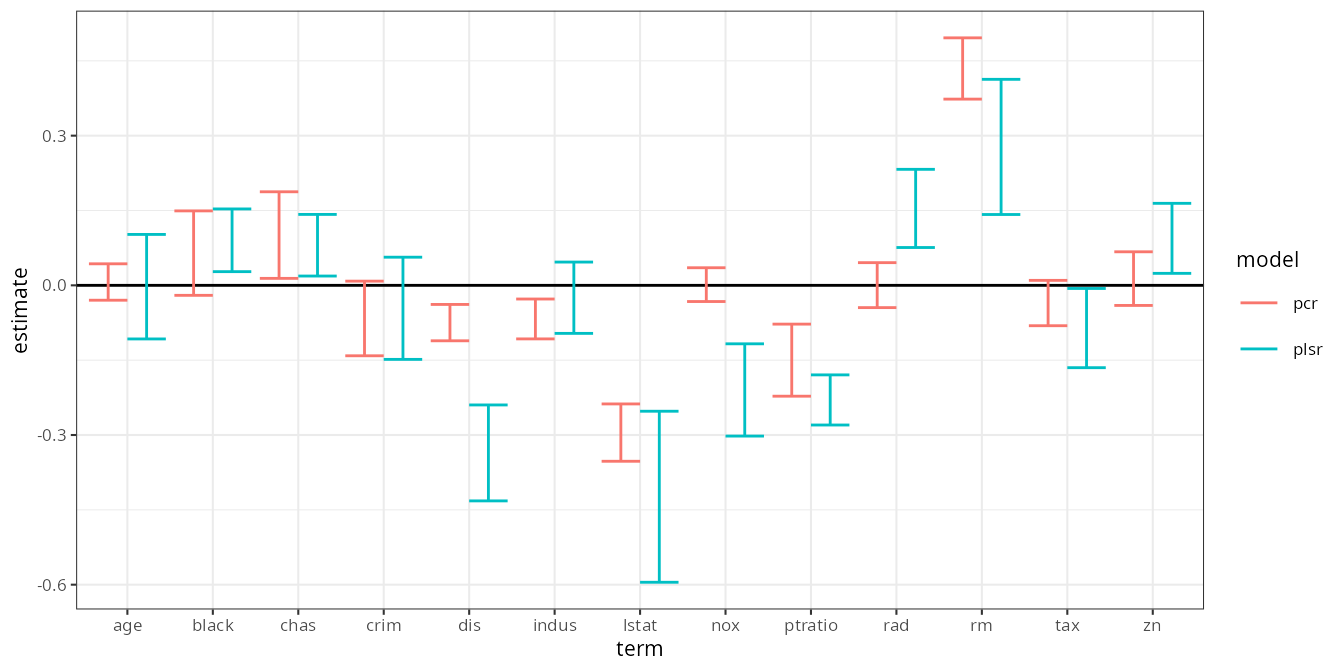

Comparing to built-in jackknife procedure

The pls-package includes built-in functionality to jackknife confidence intervals for the coefficients. We can compare these results by passing jackknife = TRUE and validation = "LOO" to m(), and setting .cv = "none" (default):

model_frame_jackknife <- data |>
  regress(medv ~ ., m("plsr", ncomp = 5, jackknife = TRUE, validation = "LOO"), 
          m("pcr", ncomp = 5, jackknife = TRUE, validation = "LOO"))

jackknife_estimates <- coef(model_frame_jackknife)

Now the coef() generic method also provides standard errors and $p$ -values for the coefficients using pls::jack.test:

jackknife_estimates <- jackknife_estimates |>
  unnest(model_info) |>
  # Create approximate 95% intervals using 2 standard deviations
  mutate(.upper = estimate + 2 * std.error, .lower = estimate - 2 * std.error)

jackknife_estimates
#> # A tibble: 28 × 9
#> # Groups:   model [2]
#>    model term       estimate ncomp std.error statistic   p.value  .upper  .lower
#>    <chr> <chr>         <dbl> <dbl>     <dbl>     <dbl>     <dbl>   <dbl>   <dbl>
#>  1 plsr  (Interce… -2.34e-16     5   NA         NA     NA        NA      NA     
#>  2 plsr  crim      -8.46e- 2     5    0.0549    -1.54   1.24e- 1  0.0253 -0.194 
#>  3 plsr  zn         1.04e- 1     5    0.0400     2.60   9.61e- 3  0.184   0.0240
#>  4 plsr  indus     -3.13e- 2     5    0.0437    -0.718  4.73e- 1  0.0560 -0.119 
#>  5 plsr  chas       8.30e- 2     5    0.0365     2.28   2.33e- 2  0.156   0.0100
#>  6 plsr  nox       -2.06e- 1     5    0.0525    -3.92   9.91e- 5 -0.101  -0.311 
#>  7 plsr  rm         2.78e- 1     5    0.0771     3.61   3.38e- 4  0.433   0.124 
#>  8 plsr  age       -2.43e- 2     5    0.0575    -0.422  6.73e- 1  0.0908 -0.139 
#>  9 plsr  dis       -3.52e- 1     5    0.0510    -6.91   1.47e-11 -0.250  -0.454 
#> 10 plsr  rad        1.73e- 1     5    0.0457     3.79   1.71e- 4  0.265   0.0817
#> # ℹ 18 more rows

The plot is almost exactly identical to the bootstrap results above:

jackknife_estimates |>
  filter(term != "(Intercept)") |>
  ggplot(aes(term, estimate, color = model)) +
  geom_hline(yintercept = 0) +
  geom_errorbar(aes(ymin = .lower, ymax = .upper), position = position_dodge()) +
  theme_bw(8)