Time-varying parameters vs. rolling windows • tidyfit

In this tutorial, I compare the coefficients estimated using a rolling window regression to those estimated using a Bayesian time-varying parameter model. For a primer on how to fit rolling window regressions using tidyfit, please see here. This articles follows directly from the linked primer, but focuses on only one industry.

library(dplyr); library(tidyr); library(purrr) # Data wrangling
library(ggplot2); library(stringr) # Plotting
library(lubridate)   # Date calculations
library(tidyfit)     # Model fitting

Load the data

data <- Factor_Industry_Returns
data <- data %>% 
  mutate(Date = ym(Date)) %>%         # Parse dates
  mutate(Return = Return - RF) %>%    # Excess return
  select(-RF)
data
#> # A tibble: 7,080 × 8
#>    Date       Industry Return `Mkt-RF`   SMB   HML   RMW   CMA
#>    <date>     <chr>     <dbl>    <dbl> <dbl> <dbl> <dbl> <dbl>
#>  1 1963-07-01 NoDur     -0.76    -0.39 -0.44 -0.89  0.68 -1.23
#>  2 1963-08-01 NoDur      4.64     5.07 -0.75  1.68  0.36 -0.34
#>  3 1963-09-01 NoDur     -1.96    -1.57 -0.55  0.08 -0.71  0.29
#>  4 1963-10-01 NoDur      2.36     2.53 -1.37 -0.14  2.8  -2.02
#>  5 1963-11-01 NoDur     -1.4     -0.85 -0.89  1.81 -0.51  2.31
#>  6 1963-12-01 NoDur      2.52     1.83 -2.07 -0.08  0.03 -0.04
#>  7 1964-01-01 NoDur      0.49     2.24  0.11  1.47  0.17  1.51
#>  8 1964-02-01 NoDur      1.61     1.54  0.3   2.74 -0.05  0.9 
#>  9 1964-03-01 NoDur      2.77     1.41  1.36  3.36 -2.21  3.19
#> 10 1964-04-01 NoDur     -0.77     0.1  -1.59 -0.58 -1.27 -1.04
#> # ℹ 7,070 more rows

We will examine only the HiTec industry to avoid unnecessary complexity:

data <- data %>% 
  filter(Industry == "HiTec") %>% 
  select(-Industry)

Model fitting

We begin by fitting a rolling window OLS regression with adjusted standard errors. In this example, we cannot simply pass both the TVP and the OLS models to the same regress function because the rolling window regression requires a .force_cv = TRUE argument, while the TVP model does not need to be fitted on rolling slices. The below code is adapted directly from the previous article on rolling window regressions:

mod_rolling <- data %>% 
  regress(Return ~ CMA + HML + `Mkt-RF` + RMW + SMB,
          m("lm", vcov. = "HAC"),
          .cv = "sliding_index", .cv_args = list(lookback = years(5), step = 6, index = "Date"),
          .force_cv = TRUE, .return_slices = TRUE)

The TVP model is fitted next. tidyfit uses the shrinkTVP package to fit TVP models. The package is extremely powerful and provides a Bayesian implementation with a specialized hierarchical prior that automatically shrinks some of the parameters towards constant processes based on the data. While I do not discuss this in more detail, have a look here for more information.

mod_tvp <- data %>% 
  regress(Return ~ .,
          m("tvp", sv = TRUE, niter = 1000, index_col = "Date"))

The sv = TRUE adds stochastic volatility, while the index_col argument is a convenience feature added by tidyfit to allow the index column (i.e. the dates) to be passed through to the estimates.

Next we combine the two model frames:

mod_frame <- bind_rows(mod_rolling, mod_tvp)

The coefficients for all models can be obtained in the usual manner:

beta <- coef(mod_frame)

Now, however, we require some wrangling to adapt the output of the two methods. First we unnest the detailed model information. This contains upper and lower credible intervals for the TVP model. For the OLS model we generate the confidence interval, as before. Finally, we combine the slice_id and index columns into a joint date column:

beta <- beta %>% 
  unnest(model_info) %>% 
  mutate(lower = ifelse(is.na(lower), estimate - 2*std.error, lower)) %>% 
  mutate(upper = ifelse(is.na(upper), estimate + 2*std.error, upper)) %>% 
  mutate(date = coalesce(as.Date(index), as.Date(slice_id)))

Plotting the results

Plotting the outcome is relatively simple with ggplot2:

beta %>% 
  ggplot(aes(date, estimate)) +
  facet_wrap("term", scales = "free", ncol = 2) +
  geom_ribbon(aes(ymax = upper, ymin = lower, fill = model), alpha = 0.25) +
  geom_line(aes(color = model)) +
  theme_bw(8)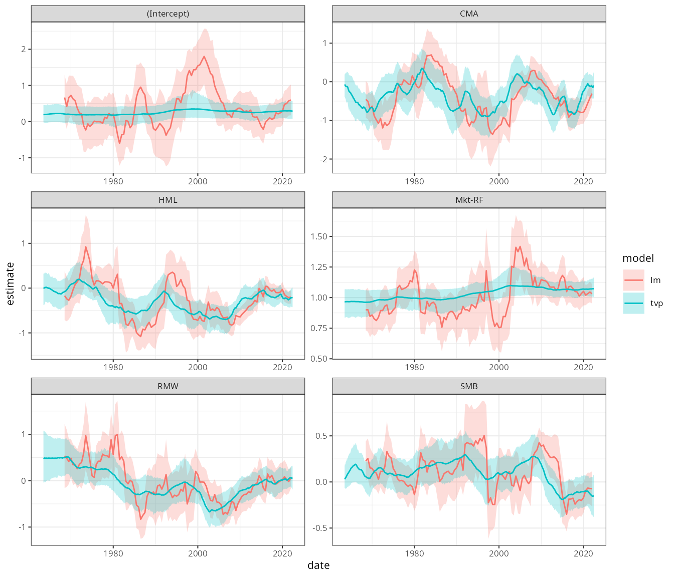

We can make a two interesting observations from these results:

The variation seen in the rolling regression for some of the parameters — specifically the risk-adjusted alpha (intercept) and the market beta — is not supported by the TVP model, which shrinks these to almost constant parameters.
The TVP estimates are markedly smoother and importantly remove the window effects seen in the rolling regression (i.e. the rolling regression adjusts too late).

The TVP model seems to offer a much better tool analyze the factor betas in this case.