Rolling Window Time Series Regression
Source:vignettes/Rolling_Window_Time_Series_Regression.Rmd
Rolling_Window_Time_Series_Regression.RmdIn this short tutorial, I show how to calculate a rolling regression
on grouped time series data using tidyfit. With very few
lines of code, we will be able to estimate and analyze a large number of
regressions. As usual, begin by loading necessary libraries:
library(dplyr); library(tidyr); library(purrr) # Data wrangling
library(ggplot2); library(stringr) # Plotting
library(lubridate)   # Date calculations
library(tidyfit)     # Model fitting
The data set consists monthly industry returns for 10 industries, as well as monthly factor returns for 5 Fama-French factors (data set is available here). The factors are:
- The market risk premium
Mkt-RF - Size
SMB(small minus big) - Value
HML(high minus low) - Profitability
RMW(robust minus weak) - Investment
CMA(conservative minus aggressive)
Returns are provided for 10 industries, and excess returns are calculated by subtracting the risk free rate from the monthly industry returns:
data <- Factor_Industry_Returns
data <- data |>
  mutate(Date = ym(Date)) |>         # Parse dates
  mutate(Return = Return - RF) |>    # Excess return
  select(-RF)
data
#> # A tibble: 7,080 × 8
#>    Date       Industry Return `Mkt-RF`   SMB   HML   RMW   CMA
#>    <date>     <chr>     <dbl>    <dbl> <dbl> <dbl> <dbl> <dbl>
#>  1 1963-07-01 NoDur     -0.76    -0.39 -0.44 -0.89  0.68 -1.23
#>  2 1963-08-01 NoDur      4.64     5.07 -0.75  1.68  0.36 -0.34
#>  3 1963-09-01 NoDur     -1.96    -1.57 -0.55  0.08 -0.71  0.29
#>  4 1963-10-01 NoDur      2.36     2.53 -1.37 -0.14  2.8  -2.02
#>  5 1963-11-01 NoDur     -1.4     -0.85 -0.89  1.81 -0.51  2.31
#>  6 1963-12-01 NoDur      2.52     1.83 -2.07 -0.08  0.03 -0.04
#>  7 1964-01-01 NoDur      0.49     2.24  0.11  1.47  0.17  1.51
#>  8 1964-02-01 NoDur      1.61     1.54  0.3   2.74 -0.05  0.9
#>  9 1964-03-01 NoDur      2.77     1.41  1.36  3.36 -2.21  3.19
#> 10 1964-04-01 NoDur     -0.77     0.1  -1.59 -0.58 -1.27 -1.04
#> # ℹ 7,070 more rows
The aim of the analysis is to calculate rolling window factor betas using a regression for each industry. To fit a regression for each industry, we simply group the data:
data <- data |>
  group_by(Industry)
Let’s verify that this fits individual regressions:
mod_frame <- data |>
  regress(Return ~ CMA + HML + `Mkt-RF` + RMW + SMB, m("lm"))

mod_frame
#> # A tibble: 10 × 7
#>    Industry model estimator_fct `size (MB)` grid_id  model_object settings
#>    <chr>    <chr> <chr>               <dbl> <chr>    <list>       <list>
#>  1 Durbl    lm    stats::lm           0.496 #0010000 <tidyFit>    <tibble>
#>  2 Enrgy    lm    stats::lm           0.496 #0010000 <tidyFit>    <tibble>
#>  3 HiTec    lm    stats::lm           0.496 #0010000 <tidyFit>    <tibble>
#>  4 Hlth     lm    stats::lm           0.496 #0010000 <tidyFit>    <tibble>
#>  5 Manuf    lm    stats::lm           0.496 #0010000 <tidyFit>    <tibble>
#>  6 NoDur    lm    stats::lm           0.496 #0010000 <tidyFit>    <tibble>
#>  7 Other    lm    stats::lm           0.496 #0010000 <tidyFit>    <tibble>
#>  8 Shops    lm    stats::lm           0.496 #0010000 <tidyFit>    <tibble>
#>  9 Telcm    lm    stats::lm           0.496 #0010000 <tidyFit>    <tibble>
#> 10 Utils    lm    stats::lm           0.496 #0010000 <tidyFit>    <tibble>
The model frame now contains 10 regressions estimated using
stats::lm. We may want to fit the regression using a
heteroscedasticity and autocorrelation consistent (HAC) estimate of the
covariance matrix, since we are working with financial time series. This
can be done by passing the additional argument to m(...):1
mod_frame_hac <- data |>
  regress(Return ~ CMA + HML + `Mkt-RF` + RMW + SMB, m("lm", vcov. = "HAC"))

mod_frame_hac
#> # A tibble: 10 × 7
#>    Industry model estimator_fct `size (MB)` grid_id  model_object settings
#>    <chr>    <chr> <chr>               <dbl> <chr>    <list>       <list>
#>  1 Durbl    lm    stats::lm           0.496 #0010000 <tidyFit>    <tibble>
#>  2 Enrgy    lm    stats::lm           0.496 #0010000 <tidyFit>    <tibble>
#>  3 HiTec    lm    stats::lm           0.496 #0010000 <tidyFit>    <tibble>
#>  4 Hlth     lm    stats::lm           0.496 #0010000 <tidyFit>    <tibble>
#>  5 Manuf    lm    stats::lm           0.496 #0010000 <tidyFit>    <tibble>
#>  6 NoDur    lm    stats::lm           0.496 #0010000 <tidyFit>    <tibble>
#>  7 Other    lm    stats::lm           0.496 #0010000 <tidyFit>    <tibble>
#>  8 Shops    lm    stats::lm           0.496 #0010000 <tidyFit>    <tibble>
#>  9 Telcm    lm    stats::lm           0.496 #0010000 <tidyFit>    <tibble>
#> 10 Utils    lm    stats::lm           0.496 #0010000 <tidyFit>    <tibble>
A rolling window regression can be estimated by specifying an
appropriate cross validation method. tidyfit uses the
rsample package from the tidymodels suite to
create cross validation slices. Apart from the classic CV methods
(vfold, loo, expanding window, train/test split), this also includes
sliding functions (sliding_window,
sliding_index and sliding_period), as well as
bootstraps. The sliding functions do not generate a
validation slice, but only create rolling window training slices. We
will be using sliding_index, which works well with date
indices. See ?rsample::sliding_index for specifics.2
Since the method lm has no hyperparameters, it is not
passed to the cross validation loop by default, since this would create
unnecessary computational overhead. To ensure that models are fitted on
train slices, we need to add the additional argument
.force_cv = TRUE. Furthermore, the CV slices are typically
not returned but only used to select optimal hyperparameters. To return
slices set .return_slices = TRUE:
mod_frame_rolling <- data |>
  regress(Return ~ CMA + HML + `Mkt-RF` + RMW + SMB,
          m("lm", vcov. = "HAC"),
          .cv = "sliding_index", .cv_args = list(lookback = years(5), step = 6, index = "Date"),
          .force_cv = TRUE, .return_slices = TRUE)
The .cv_args are arguments passed directly to
rsample::sliding_index. We are using a 5 year window
(lookback = years(5)), and skipping 6 months between each
window to reduce the number of models fitted
(step = 6).
The model frame now contains models for each slice for each industry.
The slice_id provides the valid date for the respective
slices. Betas can be extracted using the built-in coef
function:
df_beta <- coef(mod_frame_rolling)
df_beta
#> # A tibble: 6,480 × 6
#> # Groups:   Industry, model [10]
#>    Industry model term        estimate slice_id   model_info
#>    <chr>    <chr> <chr>          <dbl> <chr>      <list>
#>  1 Durbl    lm    (Intercept)  -0.434  1968-07-01 <tibble [1 × 3]>
#>  2 Durbl    lm    CMA           0.0258 1968-07-01 <tibble [1 × 3]>
#>  3 Durbl    lm    HML           0.661  1968-07-01 <tibble [1 × 3]>
#>  4 Durbl    lm    Mkt-RF        1.28   1968-07-01 <tibble [1 × 3]>
#>  5 Durbl    lm    RMW           0.898  1968-07-01 <tibble [1 × 3]>
#>  6 Durbl    lm    SMB          -0.150  1968-07-01 <tibble [1 × 3]>
#>  7 Durbl    lm    (Intercept)  -0.423  1969-01-01 <tibble [1 × 3]>
#>  8 Durbl    lm    CMA           0.235  1969-01-01 <tibble [1 × 3]>
#>  9 Durbl    lm    HML           0.569  1969-01-01 <tibble [1 × 3]>
#> 10 Durbl    lm    Mkt-RF        1.25   1969-01-01 <tibble [1 × 3]>
#> # ℹ 6,470 more rows
In order to plot the betas, we will add confidence bands. HAC
standard errors are nested in model_info in the
coefficients frame:
df_beta <- df_beta |>
  unnest(model_info) |>
  mutate(upper = estimate + 2 * std.error, lower = estimate - 2 * std.error)
df_beta
#> # A tibble: 6,480 × 10
#> # Groups:   Industry, model [10]
#>    Industry model term      estimate slice_id std.error statistic  p.value upper
#>    <chr>    <chr> <chr>        <dbl> <chr>        <dbl>     <dbl>    <dbl> <dbl>
#>  1 Durbl    lm    (Interce…  -0.434  1968-07…     0.383   -1.13   2.62e- 1 0.332
#>  2 Durbl    lm    CMA         0.0258 1968-07…     0.262    0.0985 9.22e- 1 0.550
#>  3 Durbl    lm    HML         0.661  1968-07…     0.239    2.77   7.68e- 3 1.14
#>  4 Durbl    lm    Mkt-RF      1.28   1968-07…     0.124   10.3    2.00e-14 1.52
#>  5 Durbl    lm    RMW         0.898  1968-07…     0.378    2.37   2.11e- 2 1.65
#>  6 Durbl    lm    SMB        -0.150  1968-07…     0.133   -1.13   2.65e- 1 0.116
#>  7 Durbl    lm    (Interce…  -0.423  1969-01…     0.396   -1.07   2.90e- 1 0.369
#>  8 Durbl    lm    CMA         0.235  1969-01…     0.264    0.889  3.78e- 1 0.764
#>  9 Durbl    lm    HML         0.569  1969-01…     0.243    2.34   2.29e- 2 1.06
#> 10 Durbl    lm    Mkt-RF      1.25   1969-01…     0.150    8.33   2.52e-11 1.55
#> # ℹ 6,470 more rows
#> # ℹ 1 more variable: lower <dbl>
Now, with all the pieces in place, we can plot the results. Let’s
begin by examining the market beta for each industry using
ggplot2:
df_beta |>
  mutate(slice_id = as.Date(slice_id)) |>
  filter(term == "Mkt-RF") |>
  ggplot(aes(slice_id)) +
  geom_hline(yintercept = 1) +
  facet_wrap("Industry", scales = "free") +
  geom_ribbon(aes(ymax = upper, ymin = lower), alpha = 0.25) +
  geom_line(aes(y = estimate)) +
  theme_bw(8)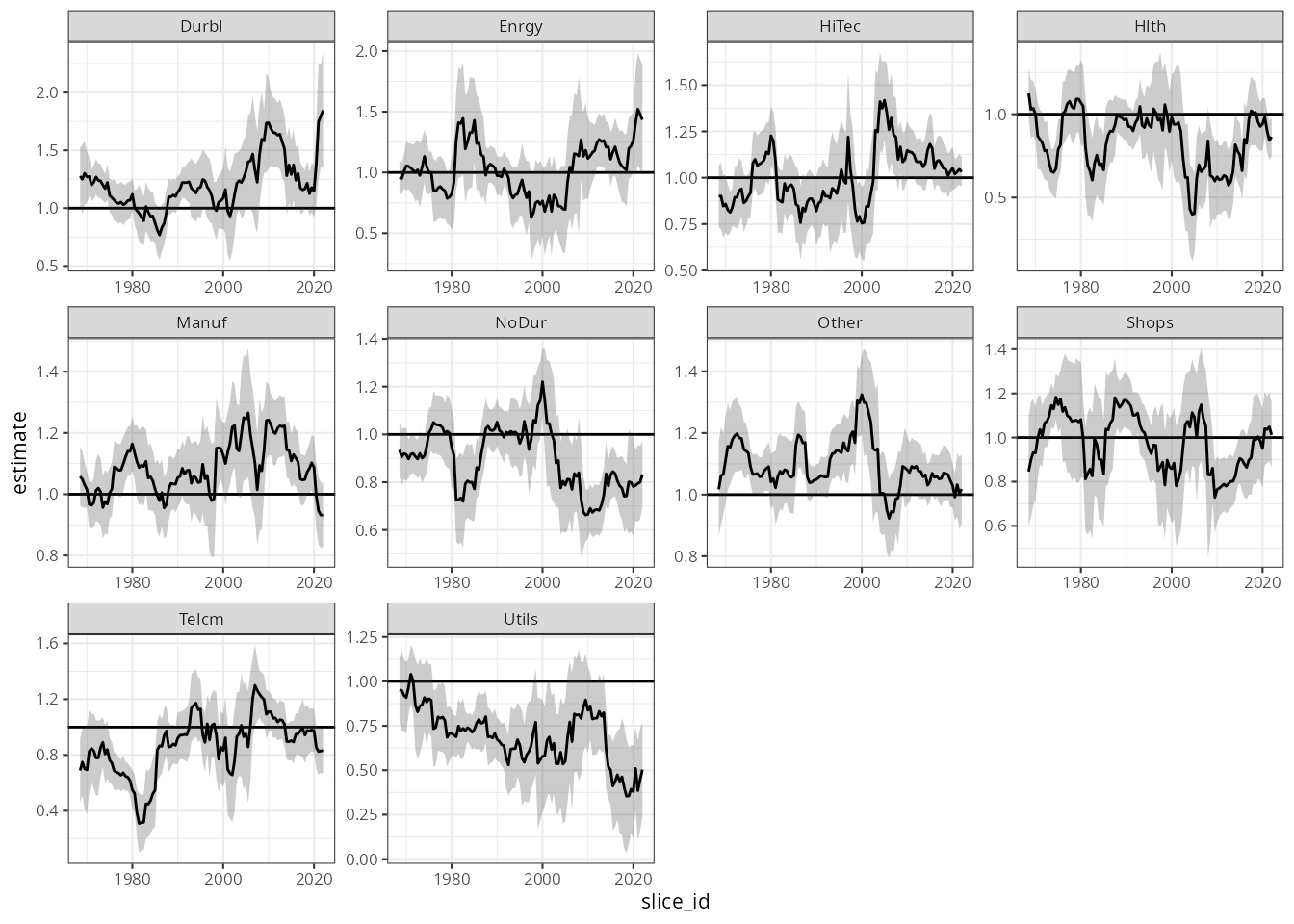
Or plotting risk-adjusted return (alpha) given by the intercept:
df_beta |>
  mutate(slice_id = as.Date(slice_id)) |>
  filter(term == "(Intercept)") |>
  ggplot(aes(slice_id)) +
  geom_hline(yintercept = 0) +
  facet_wrap("Industry", scales = "free") +
  geom_ribbon(aes(ymax = upper, ymin = lower), alpha = 0.25) +
  geom_line(aes(y = estimate)) +
  theme_bw(8)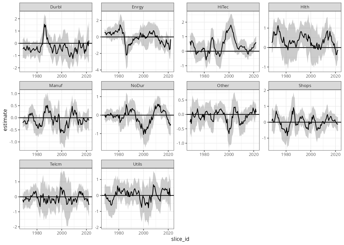
Or plotting all parameters for the HiTec industry:
df_beta |>
  mutate(slice_id = as.Date(slice_id)) |>
  filter(Industry == "HiTec") |>
  ggplot(aes(slice_id)) +
  geom_hline(yintercept = 0) +
  facet_wrap("term", scales = "free") +
  geom_ribbon(aes(ymax = upper, ymin = lower), alpha = 0.25) +
  geom_line(aes(y = estimate)) +
  theme_bw(8)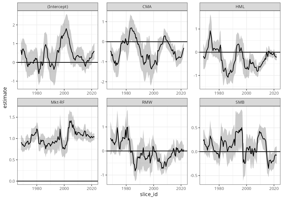
While there are certainly very interesting insights to be had here,
the aim of this walk-through is not to interpret these results, but
rather to demonstrate how a complex piece of analysis can be done very
efficiently using the tidyfit package.
In a follow-up article found here, I compare the results in the plot above to a time-varying parameter regression to show how more robust methods can be used to avoid window effects in the rolling sample and to shrink some coefficients to constant values.
Note that the
...inm()passes arguments to the underlying method (i.e.stats::lm). However in some casestidyfitadds convenience functions, such as the ability to pass avcov.argument as used incoeftestforlm.↩︎It is important to note that
sliding_indexcan not be used to select hyperparameters since no test slices are produced. To perform time series CV, use therolling_originsetting, which is similar, but produces train and test splits.↩︎